Abstract

In this slightly longer post I want to outline some of the differences in the econometric modeling techniques when the dependent variable is a binary variable with two distinct outcomes (yes/no, 0/1). We will discuss the shortcomings of ordinary least squares (OLS) in these settings and how the concept of a conditional expectation function (CEF) is replaced by the concept of a conditional probability function (CPF) that gives rise to the so called logit and probit models used for binary responses. Within these frameworks, the least squares principle is replaced by maximum likelihood estimation, which is the estimation technique common to all applications where the response variable is of qualitative nature. The theoretical discussion will be complemented with an illustrative example.

Introduction and Theory

Ordinary Least Squares (OLS) is undoubtedly the most frequently used estimation technique within the Classical Linear (Regression) Model (CLM) to recover a functional and foremost causal relationship between a dependent variable of interest $ y $ and explanatory variables (regressors) $x_j $ with $j = 1, …, k $ by means of parameter estimation. But the framework of the CLM underlies certain important assumptions for why within this framework the OLS-principle should be used only in circumstances where there are good reasons to believe that the underlying assumptions are fulfilled.

In many applications the response variable $ y $ we are trying to model is available on a continuous (or sufficiently continuous) measurement scale and in many instances also (roughly) normally distributed, at least after adequate transformations (e.g. log-transformations etc.). But this changes if we want to model categorial (or qualitative) variables, which are always discrete and can be binary/multinomial/ordered or quantitative variables with a restricted range (e.g., counts, durations, censored, truncated) that can be both, continuous or discrete. Within the class of categorial variables, the models used differ with respect to the response variable we are trying to model (hence they are called binary, multinomial or ordered response models).
Binary variables arise from the answer to yes/no questions, multinomial extends the binary variables to the setting where we have more than two mutually exclusive and exhaustive categories that cannot be ordered and finally ordered variables are like multinomial variables but with a meaningful ordering of the categories.

The OLS-principle assumes relationships between quantitative variables, where the regressors can enter the model also as dummy variables and the response is assumed to be continuous. For $i = 1, …, n$, the PRF (population regression function) for the simple linear model can be written as

$\begin{eqnarray*} y_i & = & \beta_1 + \beta_2 x_{2i} + ... + \beta_k x_{ki} + \epsilon_i \\ & = & \sum_{j=1}^K\beta_jx_{ji} + \epsilon_i \\ & = & \mathbf{x_i'\beta} + \epsilon_i. \end{eqnarray*}$

which can be compactly written as $\mathbf{y} = \mathbf{X \beta} + \mathbf{\epsilon}.$ Under the Gauß-Markov assumptions which are (1) linearity in parameters, (2) full rank of the design matrix, (3) exogeneity of the explanatory variables $ E(\mathbf{\epsilon}\vert \mathbf{X})=0 $ and homoscedastic and uncorrelated errors, meaning that the variance/covariance matrix simply is $ Cov\mathbf{(\epsilon)} = \sigma^2 \mathbf{I} $, the ordinary least squares estimator is the best linear unbiased estimator (BLUE) and we can rewrite the model in terms of the then correctly specified conditional expectation function

$\begin{eqnarray*} E(\mathbf{y}\vert \mathbf{X})=\mathbf{X\beta}, \end{eqnarray*}$

i.e., the systematic component of our linear regression model describes the conditional expectation.¹ If, in addition, we assume the errors to be normally distributed, inference based on $t $ and $F $ tests is exact.²

We could try to apply the least squares principle from above to a binary response variable $ y_i $ where the categories are coded with numerical values $0 $ and $ 1 $. And to follow the argumentation it is useful to think of the linear regression model in terms of the conditional expectation function as specified above. For a binary variable (Bernoulli variable) where $p$ is denoted as the "success probability" we know that the expectation is $E(y_i) = 0 \cdot P(y_i=0) + 1 \cdot P(y_i=1) = P(y_i=1) =p_i$, i.e., the expectation equals the success probability. And due to $Var(y_i) = E(y_i - E(y_i))^2 = E(y_i^2) - E(y_i)^2$ we get $Var(y_i) = p_i - p_i^2 = p_i(1-p_i)$. If we were to use this in a linear regression we would have $P(y = 1|\mathbf{x}) = E(y_i\vert \mathbf{x_i})=\mathbf{x_i’\beta}$ and consequently $Var(y_i\vert \mathbf{x_i})=\mathbf{x_i’\beta}(1-\mathbf{x_i’\beta})$. The problem with this specification is that $\mathbf{x_i’\hat{\mathbf{\mathbf{\beta}}}}$ (our linear predictor) is not restricted and can lead to nonsense predictions, i.e., predictions that are outside of the admissible range of [0, 1] and is therefore not well suited for modeling the success probability of our response variable $y_i$ for a specific individual or entity given a set of covariates $x_{ji}$. In addition, $Var(y_i\vert \mathbf{x_i})=\mathbf{x_i’\beta}(1-\mathbf{x_i’\beta})=p_i(1-p_i)$ shows that if $p_i$ differs across individuals (depending on our linear predictor) then also our variance is not constant but is different for every individual $i$, i.e. we have heteroscedasticity.

To overcome the difficulties, a different estimation technique is applied, namely Maximum Likelihood Estimation (MLE). In contrast to OLS, in MLE the starting point is a parametric distribution of the response variable (or the error term) where the parameters are specified as a function of the exogenous variables. By modeling the probability distribution of a response $\mathbf{y}$ conditional on regressors $\mathbf{X}$ the emphasis is shifted away from the conditional expectation function as in the OLS-framework towards the conditional probability function. This procedure can be applied to a broader class of distributions within the framework of Generalized Linear Models (GLMs) which are an extension of the classical linear regression model to accommodate both non-normal response distributions and transformations to linearity. This framework allows a unified treatment of statistical methodology for several important classes of models where the response variables have an error distribution out of the class of the exponential family which incorporates the Bernoulli, Binomial, Poisson, Gamma or inverse Normal distribution etc. The GLM thereby allows the linear predictor to be related to the response variable via a link function and allows the magnitude of the variance of each observation to be a function of its predicted value.³

GLMs

For GLMs the conditional distribution of $y_i\vert \mathbf{x_i}$ is given by a density of the following type

$\begin{eqnarray*} f(y; \theta, \phi)=exp\left(\frac{y\theta-b(\theta)}{\phi}+c(y, \phi)\right) \end{eqnarray*}$

where $ b(.) $ and $ c(.) $ are known functions and $ \theta $ and $ \phi $ are the so-called canonical and dispersion parameter.⁴ By appropriately choosing $b(.)$ and $c(.)$ it is possible to generate the different distributions (normal, binomial, Poisson, …).
To generate a regression model based on this exponential family one further states the conditional expectation to be $ \mu_i=E(y_i\vert \mathbf{x_i}) $ and the linear predictor to be $ \eta_i=\mathbf{x_i’\beta} $ which are connected via a monotone transformation $ g(\mu_i)=\eta_i=\mathbf{x_i’\beta} $ where $ g(.) $ is called link function.⁵ And because $ g(.) $ is assumed to be a monotonic function it is invertible and we can rearrange to get $ \mu_i = g^{-1}(\eta_i) = g^{-1}(\mathbf{x_i’\beta}) $. Furthermore, $ \theta $ is also an invertible function of $ \mu $ and it can be shown that $ E(y_i\vert \mathbf{x_i})=\mu_i=b’(\theta_i) $, which could be rearranged to $ \theta_i=(b’)^{-1}(\mu_i) $, and $ Var(y_i\vert \mathbf{x_i})=\phi b’’(\theta_i) $. We see that the canonical parameter $ \theta $ is connected to our conditional expectation $ \mu $ via the function $ b(.) $ and that $ E $ and $ Var $ are not completely separated but the variance is, in the general case, a function of $ \phi $ and $ \theta $, therefore the variance is also a function of our expectation $ \mu $ which is often written down as $ Var(y_i\vert \mathbf{x_i})=\phi b’’(\theta(\mu)) $ where $ V(\mu)=b’’(\theta(\mu)) $ is called the variance function. If we combine all of the above we see that

$\begin{eqnarray*} \theta_i = (b')^{-1}(\mu_i)=(b')^{-1}(g^{-1}(\mathbf{x_i' \beta})) \end{eqnarray*}$

where we see that we have multiple transformations between the linear predictor, the conditional expectation and the canonical parameter. In the linear regression model we have $ \mathbf{x_i’\beta}=\eta_i=\mu_i=\theta_i $.

A GLM for Binary Responses

To pass these concepts on to a Bernoulli-distributed random variable $ y $ which takes the value 1 with success probability $ p $ and the value 0 with probability $ (1-p) $ we can, as a first step, simply write down the probability mass function which is

$\begin{eqnarray*} f(y;\mu) = \mu^y (1-\mu)^{1-y}\!\quad \text{for }y\in\{0,1\}. \end{eqnarray*}$

This mass function⁶ can be rewritten to

$\begin{eqnarray*} f(y; \mu) & = & \mu^{y} (1-\mu)^{1-y} \\ & = & exp \left \{y \cdot log \left ( \frac{\mu}{1-\mu} \right) + log(1 - \mu) \right \} \end{eqnarray*}$

In this representation we see that $ \phi=1 $ and that $ c(y, \phi) $ is also not part of it. Comparing the remaining terms to the general representation of GLMs we see that $ \theta=log\left(\frac{\mu}{1-\mu}\right) $, i.e. our canonical parameter $ \theta $ is a function of our conditional expectation $ \mu $. Here, $ \theta $ is said to be the logit transform of $ \mu $. Solving for $ \mu $ we see that $ \mu=\frac{e^\theta}{1+e^\theta} $ and we further get $ b(\theta)=-log\left(1-\frac{e^\theta}{1+e^\theta}\right)=…=log(1+e^\theta) $. From this we can derive $ b’(\theta) = \frac{1}{1 + exp(\theta)} \cdot exp(\theta) = \mu $ and after some algebra also the variance function $ V(\mu) = b’’(\theta(\mu)) = \mu(1 - \mu) $. By this we can represent the variance function as a function of $ \mu $ instead of our canonical parameter $ \theta$⁷. So we see, that in the Bernoulli-model it holds that $ E[y_i\vert \mathbf{x_i}]=\mu_i=b’(\theta) $ and that $ Var[y_i\vert \mathbf{x_i}]=\phi \cdot V(\mu_i)=\phi \cdot b’’(\theta(\mu))=\mu_i(1-\mu_i) $, what is exactly what we postulated above. Here we clearly see how the conditional expectation \( \mu$ influences our variance.⁸

In general, each response distribution allows a variety of link functions to connect the mean with the linear predictor. In the case of binary dependent variables, the two most widely used links are the logit and the probit link⁹. For each response distribution the link function $ g=(b’)^{-1}$ for which we get \( \theta \equiv \eta$ is called the canonical link. In case of binary responses the two most widely used links are the canonical logit or probit link. From above we see that \( \theta=(b’)^{-1}(\mu)=log\left(\frac{\mu}{1-\mu}\right) $ and so the link function $ g=(b’)^{-1} $ for which we get $ \theta \equiv \eta $ is exactly $ log\left(\frac{\mu}{1-\mu}\right) $ because then $ \theta = (b’)^{-1} (g^{-1} (\mathbf{x’ \beta})) = \mathbf{x’ \beta} = \eta $. By setting $ log\left(\frac{\mu}{1-\mu}\right)=\eta $ we also see that $ \frac{\mu}{1-\mu}=exp(\eta) $ and further that $ \mu = \frac{\exp(\eta)}{1+exp(\eta)} $.

In the paragraph above we rolled up the field from behind in an attempt to show how the relevant quantities naturally arise from a Bernoulli distribution. In practice, this is of course known and therefore one can immediately summarize the relevant results as follows: a binary regression model links the conditional probability that we want to model $ \mu_i = P(y_i=1\vert \mathbf{x_i})=E(y_i\vert\mathbf{x_i}) $ to the linear predictor $ \eta_i $ via a function $ g^{-1}(.) $ which is a strict monotonic increasing distribution function so that $ g^{-1}(\eta) \in [0, 1] $ always holds and we have

$\begin{eqnarray*} \mu_i=g^{-1}(\eta_i)=g^{-1}(\mathbf{x_i'\beta}) \end{eqnarray*}$

By means of the inverse function $ g=(g^{-1})^{-1} $ it holds that $ g(\mu_i)=\eta_i=\mathbf{x_1’\beta} $. In the GLM-terminology $ g^{-1}(.) $ is called response function and $ g $ is called canonical link function. It is important to note that the response function $ g^{-1}(.) $ should be chosen such that the linear predictor is mapped to the unit interval, i.e. $ g^{-1}:\mathbf{x_i’\beta}\rightarrow[0, 1] $ and the link function accordingly maps the unit interval to the real line, i.e. $ g:[0, 1] \rightarrow \mathbb{R} $. The logit-model then arises by choosing the cumulative distribution function (CDF) of the logistic distribution

$\begin{eqnarray*} P(y_i = 1) = \mu=g^{-1}(\eta)=\frac{exp(\eta)}{1+exp(\eta)} = \Lambda(\eta) \end{eqnarray*}$

that ensures that that $ \mu $ is restricted to the interval $ [0,1] $ and the corresponding logit-link function then is

$\begin{eqnarray*} g(\mu)=log\left(\frac{\mu}{1-\mu}\right)=\eta=\mathbf{x_i'\beta}. \end{eqnarray*}$

By this one generates a linear model in the log-odds (the ratio of success probability to the probability of failure) $ log(\mu/(1-\mu)) $ and transforming by taking $ exp() $ yields

$\begin{eqnarray*} \frac{\mu}{1-\mu}=exp(\mathbf{x_i'\beta}) \end{eqnarray*}$

which shows how the covariates influence the odds $ \mu/(1-\mu) $.
Similarly also other CDFs $ F(.) $ with $ F: \mathbb{R} \rightarrow [0, 1] $ can be used as the inverse link function, the most popular being

$\begin{eqnarray*} g(\mu)=\Phi^{-1}(\mu) \end{eqnarray*}$

where $\Phi^{-1} $ is the inverse CDF of the standard normal distribution and therefore this model entered the literature as the probit model. In terms of the normal distribution we would get

$\begin{eqnarray*} P(y_i = 1) & = & \mu = g^{-1}(\eta) = \Phi(\mathbf{x_i'\beta}) = \Phi(\eta)\\ & = & \int_\infty^{\mathbf{x_i'\beta}} \! \phi(z) dz = \int_\infty^{\mathbf{x_i'\beta}} \! \frac{1}{2\pi} exp\left( \frac{-z^2}{2} \right) dz \end{eqnarray*}$

As can be seen in the Figure below, the logistic and normal CDF, i.e., the inverse link functions (response functions) that map the linear predictor to the unit interval are very similar. They are both symmetric around zero but the logistic CDF somewhat slower approaches 1 and 0 for $ \eta \rightarrow +/- \infty $ respectively.

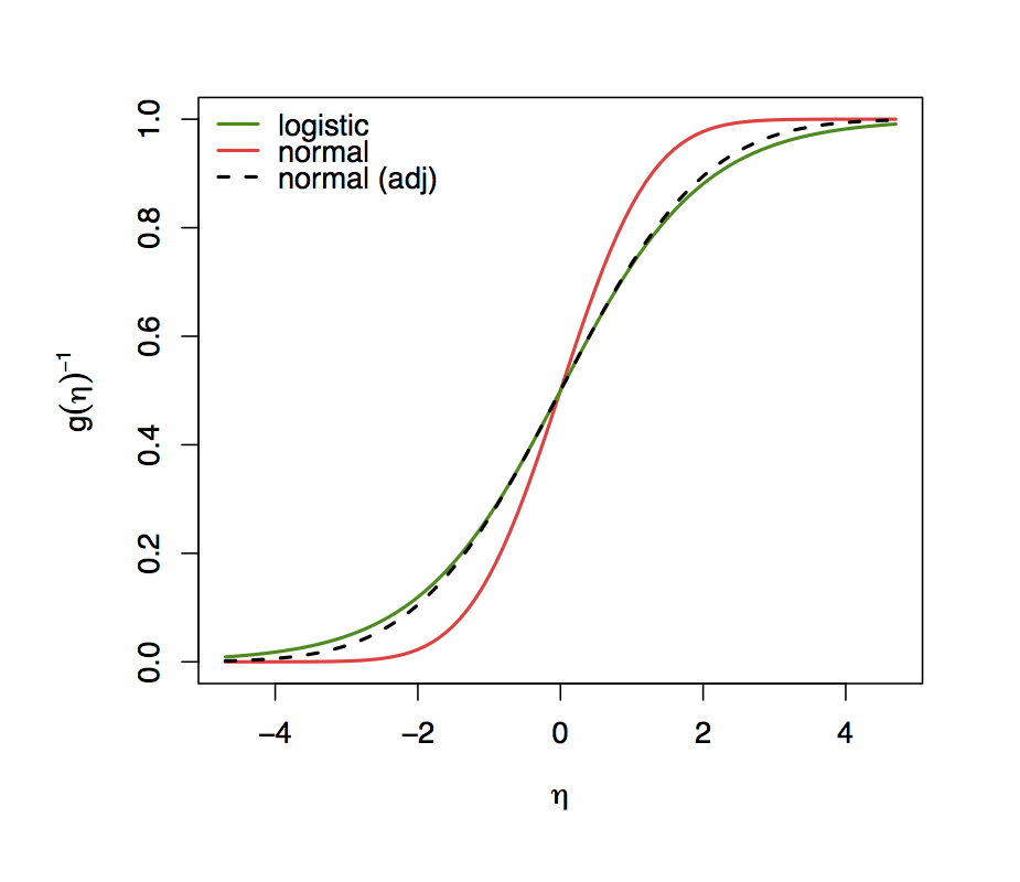Inverse Logit and Probit functions.

This emerges because the logistic distribution has somewhat heavier tails. And because the logistic CDF has a variance of $ \pi^2/3 $ (and not 1 like the standard normal distribution) it has to be compared with a rescaled normal CDF $ \Phi $ with a variance of $ \sigma^2=\phi^2/3 $. In the Figure above one can see that the Logit- and the (adjusted) Probit response function are very similar. Statistical analyses with Logit- and Probit-models therefore always lead to very similar results for the predicted probabilities. The rescaling of the parameters is thereby conserved whereby the coefficients of a Logit-models differ approximately by a factor of $ \sigma=\pi\sqrt{3} \approx 1.814 $, but the estimated probabilities are very similar.
By specifying all of the above and further assume independence (which is often natural to assume for cross-section data), we can specify the full likelihood where the parameters are connected to the linear predictor via the link-function $ g(\mu)=\eta $ and it is possible to estimate the model via maximum likelihood. For this it is important to note that the linear predictor $ \eta_i=\mathbf{x_i’\beta} $ depends on $ \beta $ and influences our conditional expectation $ \mu_i $ and further our canonical parameter $ \theta $.¹⁰ In general, there is no analytic solution to this expression and is therefore typically estimated by iterative weighted least squares which is a version of the Fisher scoring adapted to GLMs.

Latent Variable Approach

So far we have argued that we want to model probabilities therefore, statistically, it makes sense to map our linear predictor to the unit interval. Apart from these considerations there are of course also economic/behavioural justifications for why we use these specifications and the corresponding link functions. Before proceeding to these considerations we want to briefly discuss the latent variable approach.
The idea is that the binary outcomes we observe are generated by an unobservable underlying (latent) variable $ y_i $ that captures the propensity to have a "success" (i.e., outcome $ 1 $) or not. Only if this latent variable is larger than some threshold $ t $, we observe a success. This can be written down via $ y_i^* = \mathbf{x_i^\beta} + \epsilon_i $ where the linear predictor models the mean of the latent variable. But what we actually observe is only whether the latent variable exceeded some certain threshold., i.e.

$\begin{eqnarray*} y_i = I(y_i^* \geq t) = 1 \text{ if } y_i^* \geq t \text{ and } 0 \text{ otherwise } \end{eqnarray*}$

Most frequently the threshold value $ t $ is chosen to be $ 0 $ because choosing a different threshold would only affect the intercept in the estimations. The probability to have a success, i.e., that $ y_i = 1 $ for a given set of explanatory variables can then be written down as the corresponding value of the CDF evaluated at $ \mathbf{x_i’\beta} $. This can be derived via ¹¹

$\begin{eqnarray*} P(y_i = 1 | \mathbf{x_i'}) = \mu_i & = & P(y_i^* \geq 0| x_i) = P(\mathbf{x_i'\beta} + \epsilon_i \geq 0 | \mathbf{x_i})\\ & = & P(\epsilon_i \geq \mathbf{-x_i'\beta} | \mathbf{x_i}) = P(\epsilon \leq \mathbf{x_i'\beta}| \mathbf{x_i})\\ & = & F(\mathbf{x_i'\beta)} \end{eqnarray*}$

This shows that by looking at latent variables where the latent variable is explained by a mean which is the linear predictor plus some random error term we get incidental decisions ($ 0, 1 $) where the probability depends on the linear predictor and the distribution of the remaining error term around the latent variable. And then, by assuming that $ -\epsilon $ has a logistic distribution brings us to the logit model and assuming $ -\epsilon $ to be normally distributed brings us to the probit model.

MLE

Under independence, the likelihood is the product of the individual densities (i.e. the joint density, given the data) as a function of the parameter vector¹² which can be written down as ¹³

$\begin{eqnarray*} L(\theta)=L(\theta; \mathbf{y}) = \prod_{i=1}^n f(\theta; y_i). \end{eqnarray*}$

And because it is computationally easier to handle (and also numerically more stable), in practice one generally uses a log-transformation (which is monotone with respect to maximization) and writes down the log-likelihood

$\begin{eqnarray*} l(\theta)=logL(\theta) = \sum_{i=1}^n log f(\theta; y_i). \end{eqnarray*}$

where, under independence of our sample, products are turned into computationally simpler sums. Then the maximum likelihood estimator (MLE) is the parameter estimator $ \hat{\mathbf{\theta}}_{ML} $that maximizes the log-likelihood, i.e. $ \hat{\mathbf{\theta}}_{ML}=\arg\max_\theta L(\theta) = \arg\max_\theta l(\theta). $ And because the MLE depends on the specific observations (our sample) they can be considered as random variables. For inference it is then usual to look at Wald tests, Lagrange multiplier tests (LM) or Likelihood ratio (LR) tests. If GLMs are correctly specified, they inherit all properties of correctly specified ML estimation: efficiency, asymptotic normality and consistency.
Here we will not in detail discuss Maximum Likelihood theory but only write down the relevant Bernoulli likelihood that is used in estimation for binary response models and assume that the necessary regularity conditions and correct specifications of the model guarantee that our MLE is consistent, asymptotically normal and efficient.\ Assuming that the sample is i.i.d the joint distribution for the binary choice model can be written down as

$\begin{eqnarray*} Pr(\mathbf{y}|\mathbf{X}) = \prod_{i, y_i = 1} [F(\mathbf{x_i'\beta}] \prod_{i, y_i = 0} [1 - F(\mathbf{x_i'\beta})] \end{eqnarray*}$

and because the observed $ y_i $’s are the outcome of Bernoulli experiments the likelihood for a sample of $ n $ is then

$\begin{eqnarray*} L(\beta | \mathbf{y, X} = \prod_{i=1}^n [F(\mathbf{x_i\beta}]^{y_i} [1 - F(\mathbf{x_i'\beta}]^{1-y_i} \end{eqnarray*}$

where $ (.) $ again stands for either the CDF of the normal or the logistic distribution. The parameters of this model are then estimated by numerical methods (e.g. Newton-Raphson Algorithm).

Application: German Health Care Usage (GSOEP)

For our empirical application we want to make use of a dataset that is about German health care usage and originates from the German Socioeconomic Panel Survey (GSOEP). The sample covers the years 1984-95 and was used in a study by @riphahn:03 that investigated whether the presence of private insurance had an effect on the utilization (counts) of physician visits and hospital visits. The dataset is an unbalanced panel of 7,293 households and among the variables reported are household income with numerous additional sociodemographic variables including age, gender, education etc. The number of observations varies from one to seven (1,525; 1,079; 825; 926; 1,311; 1,000; 887) with a total number of 27,326 observations.¹⁴

The dataset can be used to assess various research questions with various econometric models (count data models like Poisson regression, zero-inflation models or hurdle-models; binary choice models etc.). Since we want to model binary choices, our variable of interest (dependent variable) for this application is a binary variable $y$ that indicates whether an individual visited a doctor at all or not. That is, from the potential information of counts we have in the dataset our variable $ y $ takes on only the value $ 0 $ for $ docvis=0 $ and $ 1 $ for $ docvis=1 $. From the various socioeconomic variables (covariates) we decided to use only gender, age, age2, hhinc, hhkids, educ, married and working for the regressions.

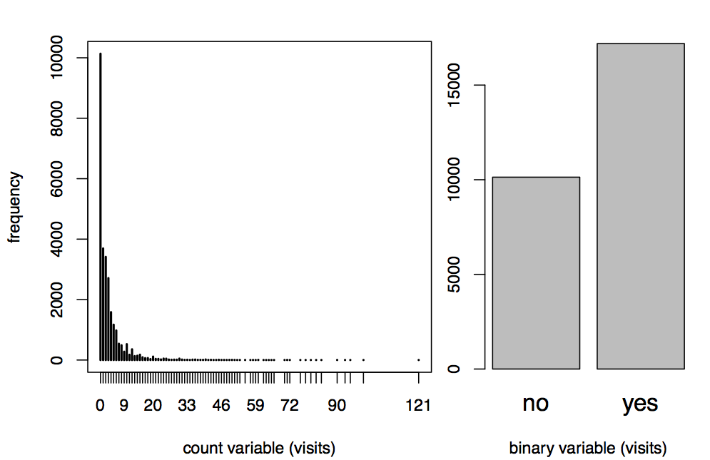Count variable of doctor visits (left), binary variable (right).

In the Figure above we can see the count variable docvis in contrast to the binary variable doc. The amount of observations that visited a doctor at least once (i.e. $y>0 $) is larger compared to observations for which we have $y=0 $. There are a total of 10,135 observations that did not visit a doctor in contrast to 17,191 that did. In the next Figure below we have also plotted the variable healthsat across gender for each level (ranging from 0 - 10). However, we have decided to not use this variable in the regressions.

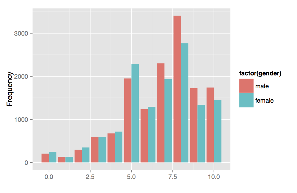Health satisfaction, coded 0 (low) - 10 (high) by gender.

Apart from the above, we can also have a look at bivariate relationships between our response and some of the regressors. In particular assessing the relationship between educ and age with our dependent variable in our Figure below, we see that with increasing education the tendency to visit a doctor decreases while with increasing age there seems to be a quadratic effect so that first the tendency to visit a doctor slightly decreases and then takes up again after the mid-fourties.

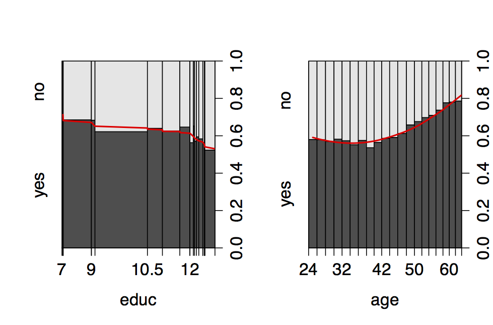Bivariate relationship between educ and age with doctor visits.

Models

As mentioned above, the dataset allows a vast array of models to be estimated. Within the binary choice models we could also make use of the panel structure of the data at hand. But due to time restrictions in preparing this project we restricted ourselves to the pooled logit and probit estimation and can hopefully add the binary models to this project anytime soon. Both models are estimated with the covariates gender, age, age2, hhinc, hhkids, educ, married and working.
The Table below reports the regression output of these two models. Looking solely at the sign of the coefficients we see that for gender: female we have a higher probability to visit a doctor, for age there are two effects (age and age2) where the coefficient for age is negative and the one for age2 positive, indicating that the probability to visit a doctor first decreases with age and then goes up again (though the effects are fairly small). For hhinc the effect is almost zero and not significant, and for hhkids: yes, educ, married: yes and working: yes the effects are significantly negative (though only on a 5% significant level for working: yes).

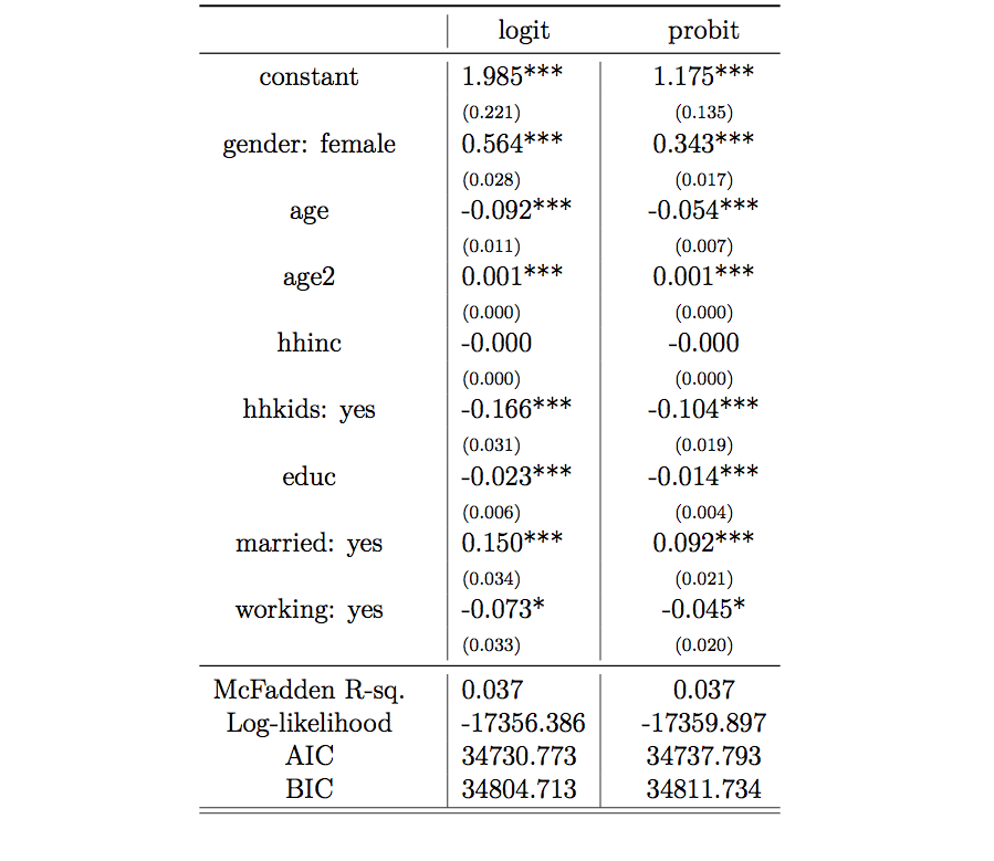Estimation results Logit and Probit.

Interpretation of Parameters

Between logit and probit models, often logit-models are preferred because, besides the latent variable approach which they have both in common, the logit-transformation has the advantage that it can be regarded as a linear model on the log-odds scale, as we have stated above. By taking expectations, i.e. $ exp(\mathbf{x_i’\beta}) $, we get a model on the odds scale, therefore the coefficients of logistic regressions can be interpreted in terms of odds. This approach makes it easy to compare two groups of subjects if they differ only for the $ lth $ regressor by one unit which then results in $ exp(\beta_l) $ and immediately states the odds ratio, which is the ratio of the respective odds between the two groups. Relative changes in the odds ratio are then simply $ exp(\beta_l) - 1 $. By this we can immediately interpret $ exp(\beta)-1 $ as changes on the odds-scale by looking at the coefficients from our logit-regression. For small $ \beta_l $ we further have $ exp({\beta_l})-1 \approx \beta_l $, c.p. For the probit model instead, a direct interpretation of the coefficients like in the logit model is not possible. Still these considerations don’t tell us something about probabilities which we actually want to model.¹⁵ For the remainder we will foremost focus on the interpretation of the logit-model (due to its interpretation in terms of odds) noting that in terms of predicted probabilities the two models are virtually equivalent.

Taking a step towards probabilities and how they are affected by changes in the regressors, things become slightly more involved than in the CLM. First of all, the estimated coefficients can be used to calculate the respective probabilities for a certain linear predictor $ \eta $, ie. for every individual in the dataset with certain characteristics there exists a corresponding (success) probability that can be computed by simply evaluating $ \hat{\mathbf{P}}r(y_i|\mathbf{x_i’}) = F(\mathbf{x_i’\hat{\mathbf{\mathbf{\beta}}}}) $. This can be, for example, used to calculate an average success probability across all individuals (which is of course not very informative as it summarizes a lot of information in the dataset). In our case the mean of the fitted probabilities (predicted probabilities) is about 0.63 (for both logit and probit). In R the predict-function can be used to compute predictions of the response $ \hat{\mathbf{\mu}}_i = \hat{\mathbf{P}}r(y_i|\mathbf{x_i’}) $ where the default is the prediction of the linear predictor. Comparing, for example, an individual with gender=male, age=44, hhinc=3500, kids=yes, educ=18, married=yes, working=yes to a person with the exact same characteristics except that we set gender=female we get a predicted probability to visit a doctor of 0.4731 as compared to 0.6123, respectively.¹⁶ The predict-function thereby takes the data and multiplies the vector of coefficients with the design matrix. By setting type = "response" the linear predictors are then automatically sent through the inverse logit link function $ \Lambda(\eta) $ that evaluates the corresponding probability.¹⁷ From these calculated probabilities it then possible to get back to the odds by plugging the calculated probabilities into the logit-link function or ($ exp(logit-link) $ function for the log-odds). So for a male person with the above stated characteristics the probability to visit a doctor are 0.8987 times the probability to not visit a doctor whereas for a female person the odds to visit a doctor are 1.578 times the probability to not visit a doctor.

For our odds-ratio (as outlined in the previous paragraph) we would get $ exp(0.564) = 1.758 $, meaning that the probability of a female person with a specific combination of covariates to visit a doctor is 1.758 times higher than the odds of a male person with exactly the same covariate values (i.e., the regressors just differ by the $lth$ regressor by one unit!). And the corresponding relative change in the odds ratio is then $ 0.7577 \approx 76\% $, meaning that the odds to visit a doctor increase by 70% by changing the $ lth$ regressor from male to female.¹⁸ Similarly we can state that if education increases by one unit we expect the odds to visit a doctor to decrease by about \( exp(-0.023) - 1 = -0.02274 = -2.274\% $, all else equal. Similarly having kids under 16 years in the household decreases the odds to visit a doctor by about 15%, being married increases them by about 14% and working decreases them by about 7% respectively. One feature of the calculation and report of odds is that they are still less well interpretable than probabilities (which are our primary interest).\ Alternatively it would also be possible to calculate the probability at the mean regressors which results in $ \hat{\mathbf{P}}r(y_i|\mathbf{\hat{\mathbf{\mathbf{x}}}_i’}) = F(\mathbf{\hat{\mathbf{\mathbf{x}}}_i’\hat{\mathbf{\mathbf{\beta}}}}) $. In our case the predicted probability at the mean regressors across the sample are 0.46 (logit) and 0.68 (probit) respectively.

In usual linear models the expectation $ E(y_i|\mathbf{x_i}) $ that we want to model is a linear function in the parameters, therefore every single parameter could be directly interpreted as a marginal effect on the expectation, ceteris paribus. An important difference of binary choice models to the CLM is that partial derivatives of the expectation, i.e. marginal effects, are not constant because they not only depend on the parameter under consideration but on the entire linear predictor that, of course, differs from person to person. This means that marginal effects result in

$\begin{eqnarray*} \frac{\partial P(y_i = 1|\mathbf{x_i'})}{\partial x_h} = \frac{\partial F(\mathbf{x_i'\beta})}{\partial\mathbf{x_h}} = f(\mathbf{x_i'\beta}) \cdot \beta_h \end{eqnarray*}$

where $ f(.) $ now stands for the derivative of either the logistic or normal CDF, i.e. the corresponding density. The factor $ f(.) $ is always positive, therefore the sign of the corresponding $ f\beta_h $ directly shows in which direction the expectation changes. Due to the non-linearity he size of a marginal effect crucially depends on the actual starting value we are considering when assessing the effect of the change of the $ lth $ regressor on the predicted probability. Depending on the individual and its characteristics (that is incorporated in the linear predictor), the marginal effect can be larger or smaller. Due to this, it is common to report "typical" effects, namely average marginal effects, similar to above where we reported average predicted probabilities and predicted probabilities at mean regressors. These can be calculated either by taking the mean over all observations (i.e. calculate the marginal effect for each observation and than take the mean) or calculate the marginal effect at the mean of the regressors. In the former case we average across the probablity-scale, in the later across the regressor-scale, therefore also the results will differ.
Because average probabilities as well as average marginal effects always merge a lot of information in one single number, their usefulness in terms of representation of the information in the data is debatable. Therefore it is often better to evaluate marginal probability effects by comparing groups in the data (here: married vs. not married, working vs. not working). Another issue is that software packages to compute marginal effects often don’t compute them correctly when there are interactions or polynomials in the model.

We have seen that both, odds and average (marginal) probabilities (effects) are either difficult to interpret or not very representative for the information in the dataset. Therefore, another very helpful tool to assess the information in the data is to fix all but the $ lth $ regressor at their mean and then evaluate the marginal probability effects for the steps in the $ lth $ regressor or directly plot the predicted probability against the entire range of values of the $ lth $ regressor. We want to show here the latter for educ which are so-called "effect-plots". Such plots can be either generated by going step by step through the respective calculations, setting up a design-matrix where all but one regressor are fixed to a "typical" value we want to investigate and then let the $ lth $ regressor "run" and see how the predicted probabilities change. That is, we look how changes in one regressor, everything else fixed, translate into effects on probabilities. So instead of looking at marginal effects (which are the derivative of our expectation = success probability) it is often more convenient to directly look at the probabilities themselves. We have done this to assess the probability to visit a doctor depending on education while keeping all other values fixed to either their mean (for numeric data) or a "typical" value (for dummies). This exercise was then replicated for the same set of values except that we changed the status of working from "yes" to "no" (red line in the plot). The result can be seen in Figure below where we see that if education runs from 7 to 18, the probability to visit a doctor decreases from slightly above 57% to about 51%. In between the function is almost linear. By changing working from "yes" to "no" shifts our line so that persons that don’t work have a higher probability (but still decreasing for increasing education) across the entire range as compared to persons that do work.¹⁹

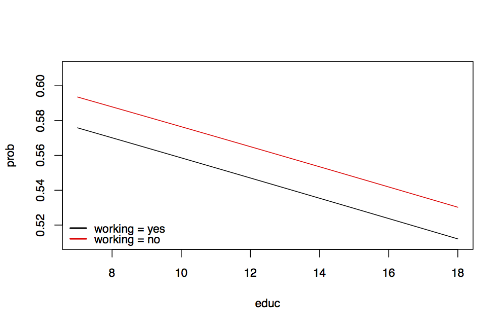Effect of education (everything else fixed at mean regressor); red line: changing “working” from “yes” to “no”.

If we want to apply the procedure above to every covariate one at a time we can use the effects-package in R that does exactly what we did automatically and generates the respective effect-plots. For this it is important to slightly adapt the function-call for the "glm" so that R recognizes that age and age2 belong together. The Figure below shows the resulting output.

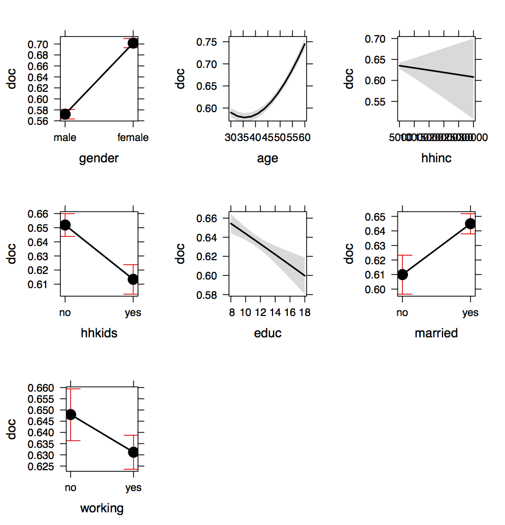Effect of education (everything else fixed at mean regressor); red line: changing “working” from “yes” to “no”.

To read these plots it is important to recognize that in each plot of the respective regressor all other covariates are fixed at their mean (or "typical") values. By this it is possible to isolate the effects of covariates on the predicted probabilities and analyze them one at a time. We see a clear difference in the probability to visit a doctor regarding gender, a quadratic age-effect whereby the probability to visit a doctor increases with age from about 37 onwards. Household income (hhinc) reflects the insignificant effect we already saw in the regression output whereas having kids that are younger than 16 (hhkids) interestingly corresponds to a slightly lower probability to visit a doctor. Education has the negative (almost linear effect) we already showed above and married individuals have, ceteris paribus, a slightly higher probability to visit a doctor whereas working individuals have a slightly lower probability to do so. Our results show that the corresponding differences in probabilities are most pronounced for the age-effect whereas for the other covariates the differences are fairly moderate.\ We want to emphasize again that for our results so far we ignored the panel-structure in the data. Our pooled logit and probit regressions are therefore just a starting point for more sophisticated binary choice panel data models.

Goodness of Fit

To assess the goodness of fit of our models there are various tools and procedures available. One option is the so-called McFadden $ R^2 $. In comparison to linear models where the $ R^2 $ is a figure that reports the proportion of the total variation in the dependent variable that is explained by the model, this variance decomposition does not work for logit/probit models. Instead, a substitute is a log-likelihood comparison of the full model (with all regressors) with a constant-only model but it cannot be interpreted as the $ R^2 $ in linear models. The McFadden $ R^2 $ is thereby calculated as

$\begin{eqnarray*} 0 \leq R_{McFadden}^2 = 1- \frac{logLik_{unrestricted}}{logLik_{restricted}} \leq 1. \end{eqnarray*}$

For the pseudo $ R^2 $ a value near one just indicates a better model fit than a value near zero. This is because if our explanatory variables have no explanatory power at all we should get $ logLik_{unrestricted} = logLik_{restricted} $ and the pseudo-$ R^2 $ would then become 0. In the extreme case where the model perfectly explains the dependent variable, the log-likelihood would be zero and the pseudo-$ R^2 $ would be 1.²⁰ In our case the corresponding values for the McFadden-$ R^2 $s are $ 0.0368 $ for the logit and $ 0.03661 $ for the probit model.

Another helpful visual tool are so-called "confusion matrices" that check the quality of the predictions in-sample. They are contingency tables of observed vs. predicted values where by choosing some cutoff probability $c$ calculated probabilities are considered a "success" or a "failure". The table summarizes correct predictions on the main diagonal and incorrect predictions on the off-diagonal. These off-diagonal values can either be "false negatives", i.e. cases that were falsely predicted to not visit a doctor while they actually did and "false positives", i.e. cases that were falsely predicted to visit a doctor while they actually didn’t. Having a look at the Table, we see that a fairly large amount of cases could be predicted accurately but unfortunately also the false negative rate is quite high with 8299 cases.²¹

Confusion Table for the Logit Model.

The last thing we did was to perform a Likelihood-Ratio test that suggests that our model is a significant improvement over a constant-only model.

Appendix

R-Code

#Econometrics Project, Binary Choice Models
#Marcel Kropp
#19.6.2014

dev.off()
## inverse logit and probit
x <- -47:47/10
par(mar = c(6, 6, 3, 3), mfrow = c(1, 1))
#quartz()
plot(x, pnorm(x), type = "l", lwd = 2,
     xlab = expression(eta), ylab = expression(g(eta)^-1),
     main = "", col = "brown1", cex.lab = 0.8, cex.axis = 0.8)
lines(x, plogis(x), lwd = 2, col = "green4")
lines(x, pnorm(x, sd = dnorm(0)/dlogis(0)), lwd = 2, lty = 2)

legend("topleft", c("logistic", "normal", "normal (adj)"),
       lty = c(1, 1, 2), lwd = 2,
       col = c("green4", "brown1", "black"),
       bty = "n", cex=0.8)




#############
## preliminaries            
#############
options(prompt = "R>", continue = "+", width = 64,
        digits = 4, show.signif.stars = TRUE)
#set.seed(1071)
getwd()
setwd("/Users/...")



#############
## original dataset            
#############
#original dataset is rather huge;
#27,326 Observations
#1 to 7 years, panel
#7,293 households observed
#The number of observations for a certain individual ranges from 1 to 7.
#Frequencies are: 1=1525, 2=2158, 3=825, 4=926, 5=1051, 6=1000, 7=987

#Here we list the variables that can be found in the complete dataset;
#The variables we used for our analysis are in CAPITAL LETTERS.

#variables:
#   ID...........person ID-number
#   FEMALE.......female = 1; male = 0
#   YEAR.........year of observation
#   AGE..........age in years
#   hsat.........health satisfaction,
#                     coded 0 (low) - 10 (high);
#                     Note, this variable has 40 coding errors.
#                     Variable NEWHSAT below fixes them.
#   handdum......handicapped = 1; otherwise = 0
#   handper......degree of handicap in percent (0 - 100)
#   DOCTOR.......1 if Number of doctor visits > 0; otherwise = 0             
#   hospital.....1 if Number of hospital visits > 0; otherwise = 0   
#   HHNINC.......household nom. month. netincome in German marks/10000
#   HHKIDS.......children under age 16 in the household = 1; otherwise = 0
#   EDUC.........years of schooling
#   MARRIED......married = 1; otherwise = 0
#   haupts.......highest degree is Hauptschul degree = 1; otherwise = 0
#   reals........highest degree is Realschul degree = 1; otherwise = 0
#   fachhs.......highest degree is Polytechnical degree = 1; otherwise = 0
#   abitur.......highest degree is Abitur = 1; otherwise = 0
#   univ.........highest degree is university degree = 1; otherwise = 0
#   WORKING......employed = 1; otherwise = 0
#   bluec........blue collar employee = 1; otherwise = 0
#   whitec.......white collar employee = 1; otherwise = 0
#   self.........self employed = 1; otherwise = 0
#   beamt........civil servant = 1; otherwise = 0
#   DOCVIS.......number of doctor visits in last three months
#   hospvis......number of hospital visits in last calendar year
#   public.......insured in public health insurance = 1;
#                otherwise = 0
#   addon........insured by add-on insurance = 1; otherswise = 0

#Notes: In the applications in the text of Greene, the following additional
#variables are used:
#   numobs.......Number of observations for this person.
#                Repeated in each row of data.
#   NEWHSAT = hsat; 40 observations on HSAT recorded between
#                   6 and 7 were changed to 7.




#############
## read in the dataset            
#############

if(!file.exists("healthcare.rda")) {
  url <- "http://people.stern.nyu.edu/wgreene/Econometrics/healthcare.csv"
  download.file(url, destfile = "healthcare.csv")
  ##read in the data into R
  healthcare <- read.csv("healthcare.csv", header = TRUE)

  ##adjust dataset
  healthcare <- subset(healthcare, select = c(id, DOCTOR, DOCVIS, NEWHSAT,
                                   EDUC, HHNINC, HHKIDS, AGE,
                                   FEMALE, MARRIED, WORKING,
                                   YEAR))
  #retransform the income variable
  healthcare$HHNINC <- (healthcare$HHNINC)*10000
  #View(healthcare)

  #further transformations; relabelling, appropriate types
  healthcare <- with(healthcare, data.frame(
    "id" = id,
    "doc" = factor(DOCTOR, levels = c(0, 1),
                   labels = c("no", "yes")),
    "docvis" = DOCVIS,
    "hsat" = NEWHSAT,
    "educ" = EDUC,
    "hhinc" = HHNINC,
    "hhkids" = factor(HHKIDS, levels = c(0, 1), labels = c("no", "yes")),
    "age" = AGE,
    "gender" = factor(FEMALE, levels = c(0, 1), labels = c("male", "female")),
    "married" = factor(MARRIED, levels = c(0, 1), labels = c("no", "yes")),
    "working" = factor(WORKING, levels = c(0, 1), labels = c("no", "yes")),
    "year" = YEAR
  ))
  ## save the file in .rda format
  save(healthcare, file = "healthcare.rda")
} else {
  load("healthcare.rda")
}


#a few separate bivariate plots
dev.off()
plot(doc ~ married, data = healthcare)
plot(doc ~ hhkids, data = healthcare)
plot(doc ~ hhinc, data = healthcare)
plot(doc ~ gender, data = healthcare)
plot(doc ~ married, data = healthcare)
plot(doc ~ working, data = healthcare)
plot(doc ~ age, data = healthcare)


#our variable of interest is the binary choice:
#visited doctor (yes/no)
barplot(table(healthcare$doc),
        xlab = "Individual visited doctor in past year",
        ylab = "absolute frequency")

#comparison reveals of count (docvis) and binary variable (doc)
layout(matrix(c(1, 2), nrow = 1), widths = c(1, 0.5))
matrix(c(1, 2), nrow = 1)
par(mar = c(4.1, 4.1, 2, 2))
plot(table(healthcare$docvis), main = "", xlab = "count variable (visits)",
                         cex.lab = 0.7, cex.axis = 0.7, ylab = "frequency")
#then we set the margins for the second graph
par(mar = c(4.1, 0.5, 2.1, 0.9))
barplot(table(healthcare$doc), xlab = "binary variable (visits)",
                         cex.lab = 0.7, cex.axis = 0.7)
table(healthcare$doc)


#health satisfaction across gender
attach(healthcare)
par(mfrow = c(1, 1))
table <- table(gender, hsat)
#reformat the data to be in long format
library("reshape2")
table.long <- melt(table, id.vars = "gender")
table.long
#use ggplot2 to create the plot
#install.packages("ggplot2")
library("ggplot2")
ggplot(table.long, aes(x=hsat, y=value, fill = factor(gender)))+
  geom_bar(stat="identity", position="dodge")+xlab("")+ylab("Frequency")


#use adapted dataset "healthcare1" for regressions
head(healthcare)
healthcare1 <- healthcare
healthcare1$docvis <- NULL
#healthcare1$hsat <- NULL
dev.off()
par(mfrow = c(1, 2))
plot(doc ~ educ, data = healthcare1, ylevels = 2:1, ylab = "", main = "")
aux <- glm(doc ~ educ + I(educ^2), data = healthcare1, family = binomial)
edu <- sort(unique(healthcare1$educ))
prop <- ecdf(healthcare1$educ)(edu)
lines(predict(aux, newdata = data.frame(educ = edu),
              type = "response") ~ prop, col = 2, lwd = 2)

plot(doc ~ age, data = healthcare1, ylevels = 2:1, ylab = "")
aux <- glm(doc ~ age + I(age^2), data = healthcare1, family = binomial)
ag <- sort(unique(healthcare1$age))
prop <- ecdf(healthcare1$age)(ag)
lines(predict(aux, newdata = data.frame(age = ag),
              type = "response") ~ prop, col = 2, lwd = 2)

#############
## models
#############
logit <- glm(doc ~ gender + age + I(age^2) + hhinc + hhkids + educ +
                   married + working,
                   family = binomial(link = "logit"),
                   data = healthcare1)
summary(logit)                               
probit <- glm(doc ~ gender + age + I(age^2) + hhinc + hhkids + educ +
                    married + working,
                    family = binomial(link = "probit"),
                    data = healthcare1)
summary(probit)
#Coefficients for probit and logit should differ by a factor of approx. 1.6
cbind(coef(logit), coef(probit)*1.6)
#install.packages("memisc")
library("memisc")
mtable(logit, probit)
toLatex(mtable(logit, probit))



#############
## predictions and
## interpretations
#############
#use predict function to compute predicted probabilities
predict(logit, data.frame(gender = "male", age = 44, hhinc = 3500, hhkids = "yes",
                          educ = 18, married = "yes", working = "yes"),
                          type = "response")
predict(logit, data.frame(gender = "female", age = 44, hhinc = 3500, hhkids = "yes",
                          educ = 18, married = "yes", working = "yes"),
                          type = "response")
predict(probit, data.frame(gender = "male", age = 44, hhinc = 3500, hhkids = "yes",
                          educ = 18, married = "yes", working = "yes"),
                          type = "response")
predict(probit, data.frame(gender = "female", age = 44, hhinc = 3500, hhkids = "yes",
                          educ = 18, married = "yes", working = "yes"),
                          type = "response")
#the relation between link-scale and probability scale can be assessed via
predict(logit, data.frame(gender = "male", age = 44, hhinc = 3500, hhkids = "yes",
                          educ = 18, married = "yes", working = "yes"),
                          type = "link")
mu1 <- exp(-0.1077)/(1+exp(-0.1077))
mu1 #is the same value that we got when setting type = "response"!

#equivalently
predict(logit, data.frame(gender = "female", age = 44, hhinc = 3500, hhkids = "yes",
                          educ = 18, married = "yes", working = "yes"),
                          type = "link")
mu2 <- exp(0.4568)/(1+exp(0.4568))
mu2

#a male person with the above covariates the probability to visit a
#doctor (yes/no) is 0.8987 times the probability to not visit a doctor.
mu1/(1-mu1) #odds
log(mu1/(1-mu1)) #log Chancen

#a female person with the above covariates the probability to visit a
#doctor (yes/no) is 1.578 times the probability to not visit a doctor.
mu2/(1-mu2) #odds
log(mu2/(1-mu2)) #log Chancen

#odds ratios (ratio of odds for female vs odds for male)
exp(0.564)
exp(0.564) - 1

#similarly:
#education
exp(-0.023) - 1

exp(-0.166) - 1 #hhkids
exp(0.150) -1 #married
exp(-0.073) - 1 #working

#all at once
as.numeric(round(exp(coef(logit)) - 1, 2))


#age is more difficult to interpret due to the quadratic term!
#also hhinc is not reported because it is insignificant and
#virtually zero!



#average predicted probabilities:
mean(predict(logit, type = "response"))
mean(predict(probit, type = "response"))


#predicted probability evaluated at mean regressors
(pred.l <- as.numeric(plogis
         (coef(logit)[1] +
         coef(logit)[2]*(length(gender[gender == "female"])/length(gender) +
         coef(logit)[3]*mean(healthcare1$age) +
         coef(logit)[5]*mean(healthcare1$hhinc) +
         coef(logit)[6]*(length(hhkids[hhkids == "yes"])/length(hhkids)) +
         coef(logit)[7]*mean(healthcare1$educ) +
         coef(logit)[8]*(length(married[married == "yes"])/length(married)) +
         coef(logit)[9]*(length(working[working == "yes"])/length(working))))))
(pred.p <- as.numeric(pnorm
         (coef(probit)[1] +
         coef(probit)[2]*(length(gender[gender == "female"])/length(gender) +
         coef(probit)[3]*mean(healthcare1$age) +
         coef(probit)[5]*mean(healthcare1$hhinc) +
         coef(probit)[6]*(length(hhkids[hhkids == "yes"])/length(hhkids)) +
         coef(probit)[7]*mean(healthcare1$educ) +
         coef(probit)[8]*(length(married[married == "yes"])/length(married)) +
         coef(probit)[9]*(length(working[working == "yes"])/length(working))))))


#calculation for effects for education "by hand"
x.matrix <- model.matrix(logit)
head(x.matrix)

xbar <- colMeans(x.matrix[, 2:9])
xbar
class(xbar)

xbar <- as.data.frame(t(xbar))
xbar

names(xbar)[1] <- "gender"
names(xbar)[5] <- "hhkids"
names(xbar)[7] <- "married"
names(xbar)[8] <- "working"
xbar
class(xbar)

xbar$gender <- replace(xbar$gender, xbar$gender=="0.47877479323721", "male")
xbar$hhkids <- replace(xbar$hhkids, xbar$hhkids=="0.402730000731904", "no")
xbar$married <- replace(xbar$married, xbar$married=="0.758618165849374", "yes")
xbar$working <- replace(xbar$working, xbar$working=="0.677047500548928", "yes")
xbar

predict(logit, xbar, type = "response")
#fixing all covariates at their mean, the "typical" person has a probability to
#visit a doctor of about 55%.

#replicate the data
xbar <- do.call("rbind", replicate(111, xbar, simplify = FALSE))
head(xbar)
summary(xbar)
#then instead of having the mean value for "education" in every row we let
#education run from 7 to 18 in steps of 0.1
educ <- seq(7, 18, by = 0.1)
xbar$educ <- educ
xbar
#all other values are fixed on a "typical" value

#then we can say again
predict(logit, xbar, type = "response")
#and calculated probabilities for a running value of "education"

xbar$prob <- predict(logit, xbar, type = "response")
xbar
#then we can write
dev.off()
plot(prob ~ educ, data = xbar, type = "l", ylim = c(0.51,0.61), cex.axis = 0.7,
     cex.lab = 0.7)
#and see that if education runs from 7 to 18, the probability to visit a doctor
#decreases from slightly above 57% to about 51%. In between the function is almost
#linear!


#the whole calculations can now be repeated for "working = no" and the line be
#added to our plot via
x.matrix <- model.matrix(logit)
head(x.matrix)

xbar <- colMeans(x.matrix[, 2:9])
xbar
class(xbar)

xbar <- as.data.frame(t(xbar))
xbar

names(xbar)[1] <- "gender"
names(xbar)[5] <- "hhkids"
names(xbar)[7] <- "married"
names(xbar)[8] <- "working"
xbar
class(xbar)

xbar$gender <- replace(xbar$gender, xbar$gender=="0.47877479323721", "male")
xbar$hhkids <- replace(xbar$hhkids, xbar$hhkids=="0.402730000731904", "no")
xbar$married <- replace(xbar$married, xbar$married=="0.758618165849374", "yes")
xbar$working <- replace(xbar$working, xbar$working=="0.677047500548928", "no")
xbar

predict(logit, xbar, type = "response")
xbar <- do.call("rbind", replicate(111, xbar, simplify = FALSE))
head(xbar)
summary(xbar)
educ <- seq(7, 18, by = 0.1)
xbar$educ <- educ
xbar
predict(logit, xbar, type = "response")
xbar$prob <- predict(logit, xbar, type = "response")
xbar
lines(prob ~ educ, data = xbar, type = "l", col = "red")
legend("bottomleft", c("working = yes", "working = no"),
       lty = c(1, 1), lwd = 2, col = c("black", "red"), bty = "n", cex=0.7)
#and see that if education runs from 7 to 18, the probability to visit a doctor
#decreases from slightly above 57% to about 51%. In between the function is almost
#linear!


#effects plots with the effects-package
#install.packages("effects")
library("effects")
#to use the effects plot we restrict ourselves to the logit-model and reestimate
#it so that R understands that "age" and "age^2" belong to one and the same
#variable. this is done via "poly()"
logit.2 <- glm(doc ~ gender + poly(age, 2, raw = TRUE) + hhinc + hhkids +
                   educ + married + working,
                   family = binomial(link = "logit"),
                   data = healthcare1)
logit.eff <- allEffects(logit.2)
plot(logit.eff, aks = FALSE, rescale.axis = FALSE, cex.axis = 0.7, cex.lab = 0.7,
     main = "", rug = FALSE)


#############
## goodness of fit
#############
#McFadden R^2
#Calculations:
#evaluating the constant-only model:
logit0 <- glm(doc ~ 1, data = healthcare1, family = binomial(link = "logit"))
logLik(logit0)
probit0 <- glm(doc ~ 1, data = healthcare1, family = binomial(link = "probit"))
logLik(probit0)

#the log-likelihood values from the unrestricted (full) model from above:
logLik(logit)
logLik(probit)


rsq.logit <- as.numeric(1-(logLik(logit)/logLik(logit0)))
rsq.logit
rsq.probit <- as.numeric(1-(logLik(probit)/logLik(probit0)))
rsq.probit


#Alternative Approach
## "Proportion of Correct Predictions"
#with cut-off value 50%
conftab1 <- table(true = healthcare1$doc, pred = fitted(logit) > 0.5) #Kreuztabelle
#confusion-Matrix mit logit
conftab2 <- table(true = healthcare1$doc, pred = fitted(probit) > 0.5) #Kreuztabelle
#confusion-Matrix mit probit
mtable(conftab1, conftab2)
toLatex(mtable(logit, probit))


#install.packages("ROCR")
library(ROCR)
pred <- prediction(fitted(logit), healthcare1$doc)
plot(performance(pred, "acc"))
plot(performance(pred, "tpr", "fpr"))
abline(0, 1, lty = 2)


##############
## LR-Test
##############
#Likelihood Ratio test: raw calculations
as.numeric(-2*(logLik(probit0)-logLik(probit))) #result: 1319 (relevant test
#statistic)
as.numeric(-2*(logLik(logit0)-logLik(logit))) #result: 1326
qchisq(0.99, 8) #we have 8 degress of freedom
#-> Hypothesis that the two models are the same can be rejected!


#LR-test with package:
#install.packages("lmtest")
library(lmtest)
lrtest(probit0, probit)
lrtest(logit0, logit)

Footnotes

This can be derived from $ E[\mathbf{y}\vert \mathbf{X}]=E[\mathbf{X\beta+\epsilon}\vert \mathbf{X}]=E[\mathbf{X\beta\vert X}]+E[\mathbf{\epsilon\vert X}]=\mathbf{X\beta}$. ↩
Note that normality of the errors is not necessary for the tests to hold and also not part of the Gauß-Markov-assumptions. ↩
Generalized linear models were formulated by @nelder:72 as a way of unifying various other statistical models, including linear regression, logistic regression and Poisson regression. ↩
If the dispersion parameter $ \phi $ is fixed then this type of distributions are called an exponential family. ↩
Due to $g(\mu_i)=\eta_i=\mathbf{x_i’\beta} $ we have $\mu_i=g^{-1}(\eta_i)=g^{-1}(\mathbf{x_i’\beta}) $ where $g^{-1} $ is the inverse link function. ↩
Here we denote the conditional expectation $ \mu $ as our success probability $ p $ which is $ \in[0, 1] $. ↩
It is important to note that $ b(.) $ is a function of $ \theta $ in the first place so that we have to differentiate with respect to $ \theta $ and not $ \mu $. ↩
In the case of the normal distribution mean and variance are independent. ↩
Details will follow below. ↩
In the setting of GLMs the dispersion parameter $ \phi $ can be treated as a nuisance parameter or is known anyway. ↩
Whereby $ F(.) $ can then be either the CDF of the normal or the logistic distribution. ↩
Switching from "likelihood" to "densities" emphasizes the reversed roles of the data and the parameters (i. e., the arguments) and is also expressed notationally by switching from the joint distribution as the joint probability density for observing $ y_1, …, y_n $ given ( \theta \) to the likelihood function of the unknown parameter $ theta $ given a random sample $ y_1, …, y_n $. ↩
Here write down the setup without regressors; the general considerations are the same for cases where we specifically consider regressors, i.e. for $ f(\theta; y_1, …, y_n\vert\mathbf{x}) $. ↩
A detailed list with the variables and their description can be found in the accompanying R code in the Appendix below. ↩
The logit model can therefore be interpreted as a semi-logarithmic model for the odds. ↩
Evaluating the predicted probabilities using the probit model instead results in virtually no difference. ↩
The default would be type = "link" that reports the corresponding value on the link-scale. ↩
Note that these odds ratios don’t change, i.e., the remain constant even if we change the other regressors, whereas the difference on the probability scale is not the same. ↩
Note that the calculations were made only using the logit-model. Applying the procedure to probit-models would result in virtually identical results. ↩
The pseudo-$ R^2 $ uses the same information as the likelihood ratio test. ↩
It is also possible to check for which cutoff-value the proportion of correct predictions is largest (see the R-Code in the Appendix below). ↩